Team Members:
Anjana Nandagopal, Elvan Ugurlu, Fereshteh Shahmiri, Serhat Erdogan, Sukris Vong.
Introduction
Motivation
The emergence of the 2019 novel coronavirus (2019-nCoV) has caused a large global outbreak and major public health issues 15. Viral pneumonia, difficulty in breathing and dyspnea became known as key symptoms in infected patients and in severe cases caused uncountable deaths since the virus outbreak 32. These circumstances that have dramatically impacted all aspects of our lives highlight the importance of early and automated diagnosis of such respiratory disorders more than ever. Moreover, it emphasized the necessity of telemedicine and smart telediagnosis of disease while the availability of professional physicians are low and the risk of in-person check outs are high.
The current situation has highly motivated us to consider our project as an opportunity to develop a telemedicine platform for remote, automated diagnosis of adventitious pathological sounds which can contribute to diagnosis of respiratory disorders. Our system may provide a better chance of benefiting from treatments as well as preventing the spread of the coronavirus. Moreover, in a broader context, it can assist pulmonologists to diagnose varying degrees of sound abnormalities and lung ailments including asthma, chronic obstructive pulmonary disease, pneumonia, infection, and inflammation of the airways and facilitate the long-term, remote monitoring and treatments in inexpensive, non-invasive, and safe ways.
Objective
In those COVID-19 cases, in which the infection has led to acute respiratory distress 14’ 32, breathing appears as distant sounds accompanied by coarse crackles and diffuse wheezes 5 ‘ 20. Besides, most respiratory ailments are accompanied by the same sound anomalies during the patient’s inspiration and/or expiration cycles 23. Thus, the key fundamental, initial step in developing our telemedicine platform is to determine the presence of adventitious sounds and distinguish between four classes of wheeze, crackle, a combination of both, and normal breathing.
Background: Respiratory Sounds
Normal and Abnormal Lung Sounds
Vesicular or normal lung sounds are usually soft and low-pitched and heard during auscultation of the chest and lung surface of a healthy person. The sounds have more distinguishable features during inspiration period than the exhalation. This is generated by turbulent airflow within the lobes of the lungs. During expiration the sound becomes softer as air flows within the larger airways. The inhalation process is normally 2-3 times the length of the exhalation process 7’ 22. On the other hand, adventitious or abnormal lung sounds consist of additional audible sounds during auscultation. This includes abnormal lung sounds such as crackles, wheezes, rhonchi, and stridor. In this project, our focus would only be on wheeze and crackle. The type, duration, location, and intensity of each adventitious breath sounds can help classify signals 4’ 8’ 17‘19.
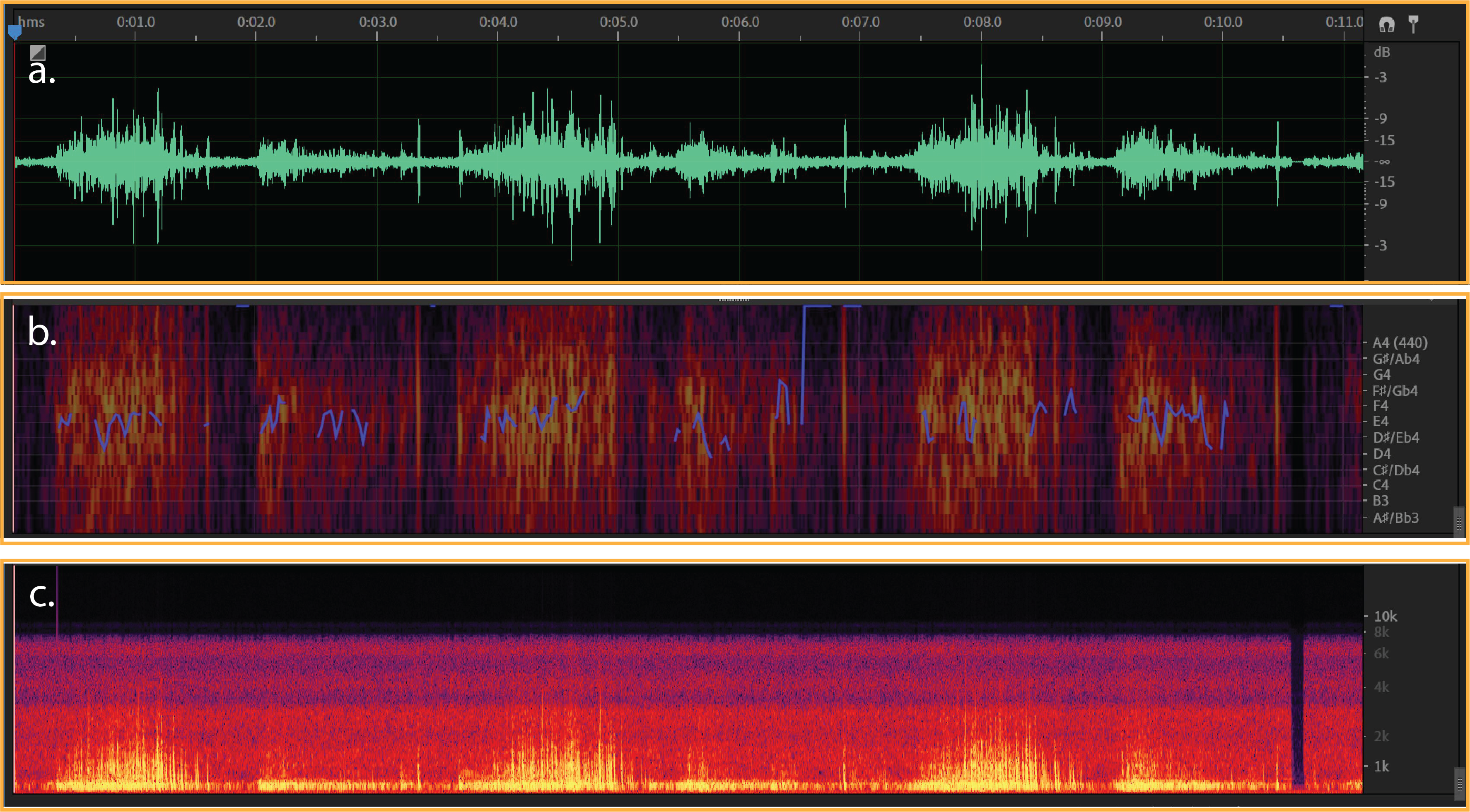
Figure 1:
a) Typical waveform from normal breath - (dB/milisecond). It shows a typical respiratory cycle with time duration about 35 milisecond.
b & c) Spectral Pitch & Frequency spectrogram for a normal breath (Hz/milisecond).
Wheeze
Wheezes are continuous, high-pitched adventitious lung sounds with the typical frequency range from 100 Hz to 5000 Hz and duration above 40 milisecond. Wheezes commonly occur at the end of the inspiratory phase or early expiratory phase as a result of the gradual opening or closing of a collapsed airway. They sound like a whistle when you breathe and are most audible during the expiratory phase. Aside from narrowed airways, wheezes can also be caused by inflammation secondary to asthma and bronchitis. If bilateral wheezing is heard in both lungs, this is an indication of bronchoconstriction. When wheezes are heard in only one lung this is referred to unilateral wheezing which indicates that a forigen body obstruction is presented 12’ 16.
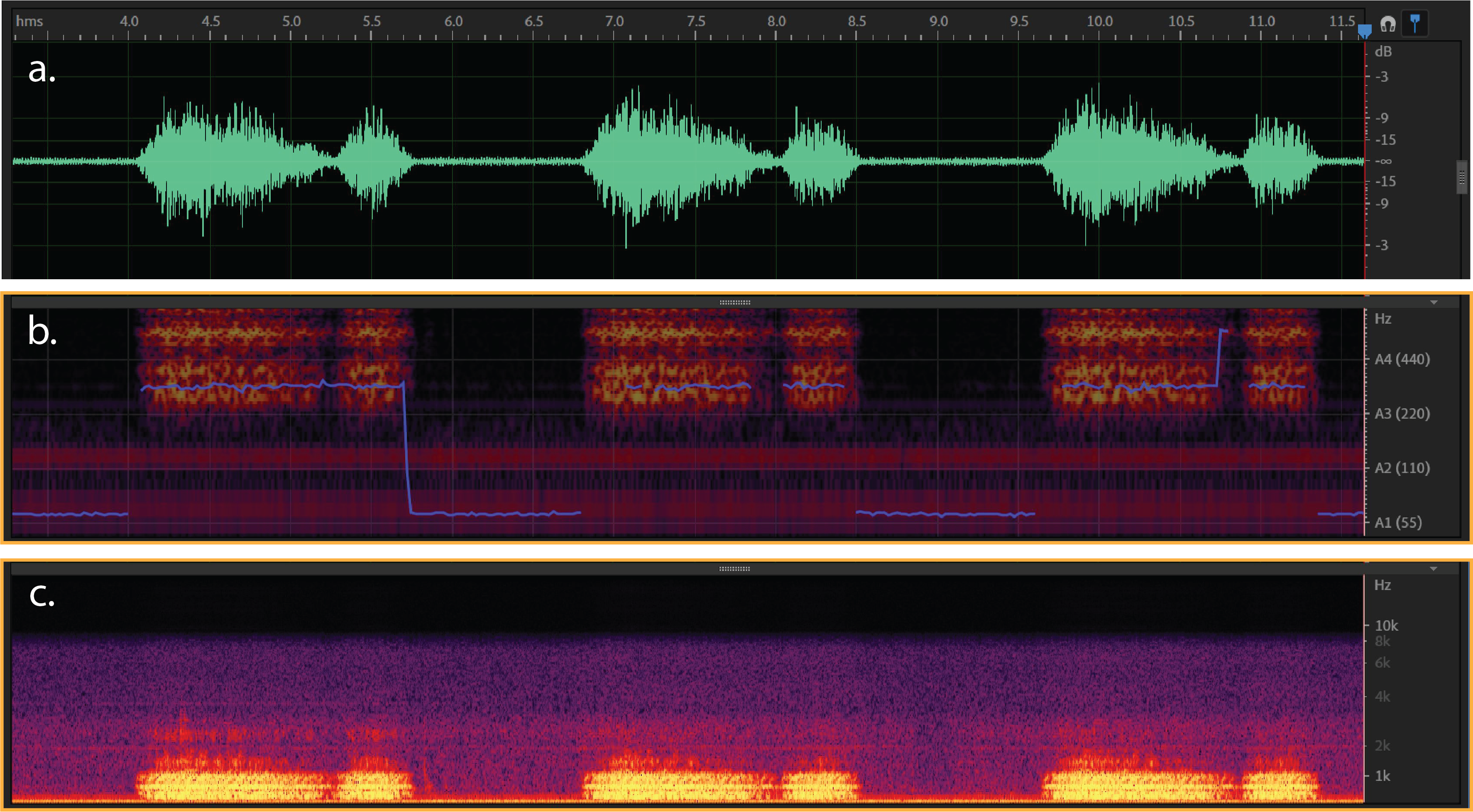
Figure 2:
a) Typical waveform from wheeze- (dB/milisecond). It shows a respiratory cycle with time duration about 40 milisecond.
b & c) Spectral Pitch & Frequency spectrogram for a wheeze sound (Hz/milisecond).
Crackles
Crackles are discontinuous, short, explosive, lung adventitious sounds in the lung fields that have fluid in the small airways. Crackles can occur on both inspiration and expiration but are more common during the inspiratory phase. There are two types of fine and coarse crackles. The fine crackles are about 650 Hz and at least minimum time duration about 5 milisecond. While the frequency of the coarse crackles is about 350 Hz and the minimum duration about 14 miliseconds. Such frequency and time ranges shows that difference between the two is that fine crackles have a higher frequency and a shorter duration and are caused by a sudden opening of a narrowed or closed airway. The sound of fine crackles can be compared to that of salt heated on a frying pan. Coarse crackles, on the other hand, are louder, lower in pitch and last longer. They are caused by secretions in the airways. The sound of coarse crackles is like pouring water out of a bottle. Crackles are often associated with lung inflammation or infection like Cronic Obstructive Pulminary Disease (COPD), chronic bronchitis, pneumonia, and pulmonary fibrosis 10’ 29.
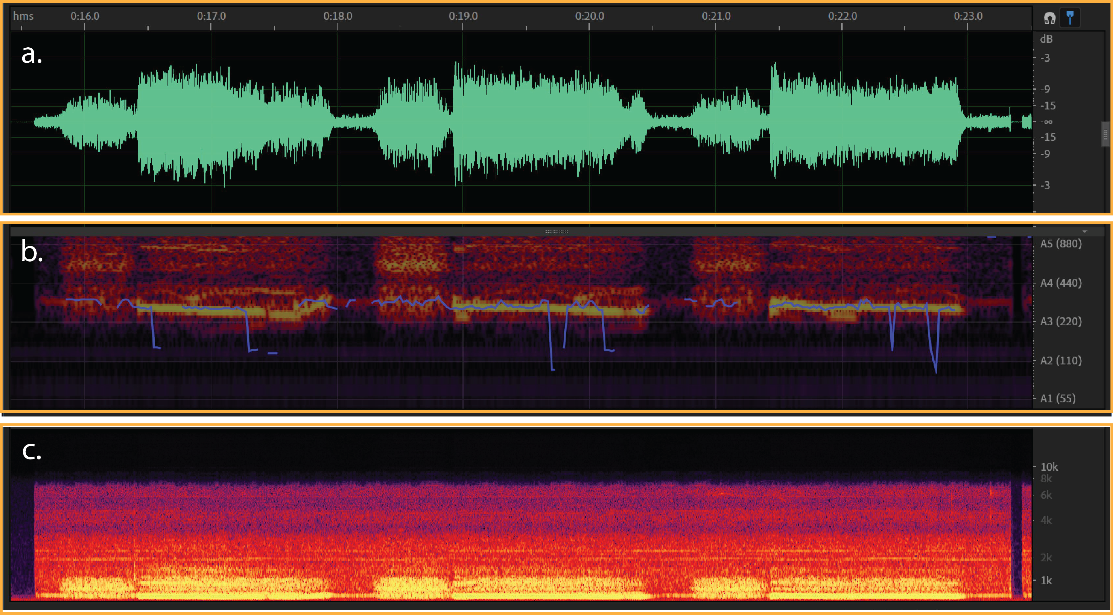
Figure 3:
a) Typical waveform from crackle- (dB/milisecond). It shows a respiratory cycle with time duration about 50 milisecond.
b & c) Spectral Pitch & Frequency spectrogram for a crackle sound (Hz/milisecond).
Overview of Data and Applied Methods in Literature
Initially we explored the literature to see how such study is typically done. The main purpose of using the “Respiratory Sound” dataset (which we will explain in next part) is to build a model to classify healthy vs unhealthy lung sounds, or to build a model to classify respiratory diseases through detection of sound anomalies2’ 3’ 9’ 18’ 27. The machine learning pipeline that most of existing projects have used include three phases. First one is preprocessing of respiratory sound through noise reduction and audio filtering techniques. The second step is feature extraction using signal processing methods like spectral analysis, cepstral analysis, wavelet transforms, and statistics. And the third step is classification, in which Artificial Neural Networks 3’ 9’ 13’ 21’ 26’ 30, Support vector machines 1, K-nearest Neighbors 25, and Gaussian Mixture models 25 have been the most popular used classifiers.
The most promising outcome is related to those projects which have used MFCC as one of the main feature extraction methods for audio data and got the best accuracy results from Neural Network based classifications. After an exploratory study in literature, we believe our approach in classifying respiratory sounds consists of three phases; 1. Again preprocessing of the audio signals, and taking advantage of both supervised and unsupervised learnings. To the best of our knowledge, there is not a study that uses the (Mel Frequency Cepstral Coefficients) MFCC features to classify the adventitious sounds into the specified four classes using SVM or CNN. In the light of similar works, we expect to achieve better results with the CNN based approach than the SVM approach as CNN approach is expected to learn the underlying distinctive features better than the SVM.
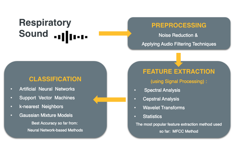
Figure 4: Workflow from preprocessing to classification
Data
Data is taken from the Respiratory Sound Database, created by two research teams in Portugal and Greece 24 . It consists of 920 recordings. Each recording varies in length. A histogram of the length of recordings is given in Figure 5. Recordings were taken from 126 patients and each recording is annotated. Annotations are comprised of beginning and end times of each respiratory cycle and whether the cycle contains crackle and/or wheeze. Crackles and wheezes are called adventitious sounds and the presence of them is used by health care professionals when diagnosing respiratory diseases. The number of respiratory cycles containing each adventitious cycle is shown in Figure 6.
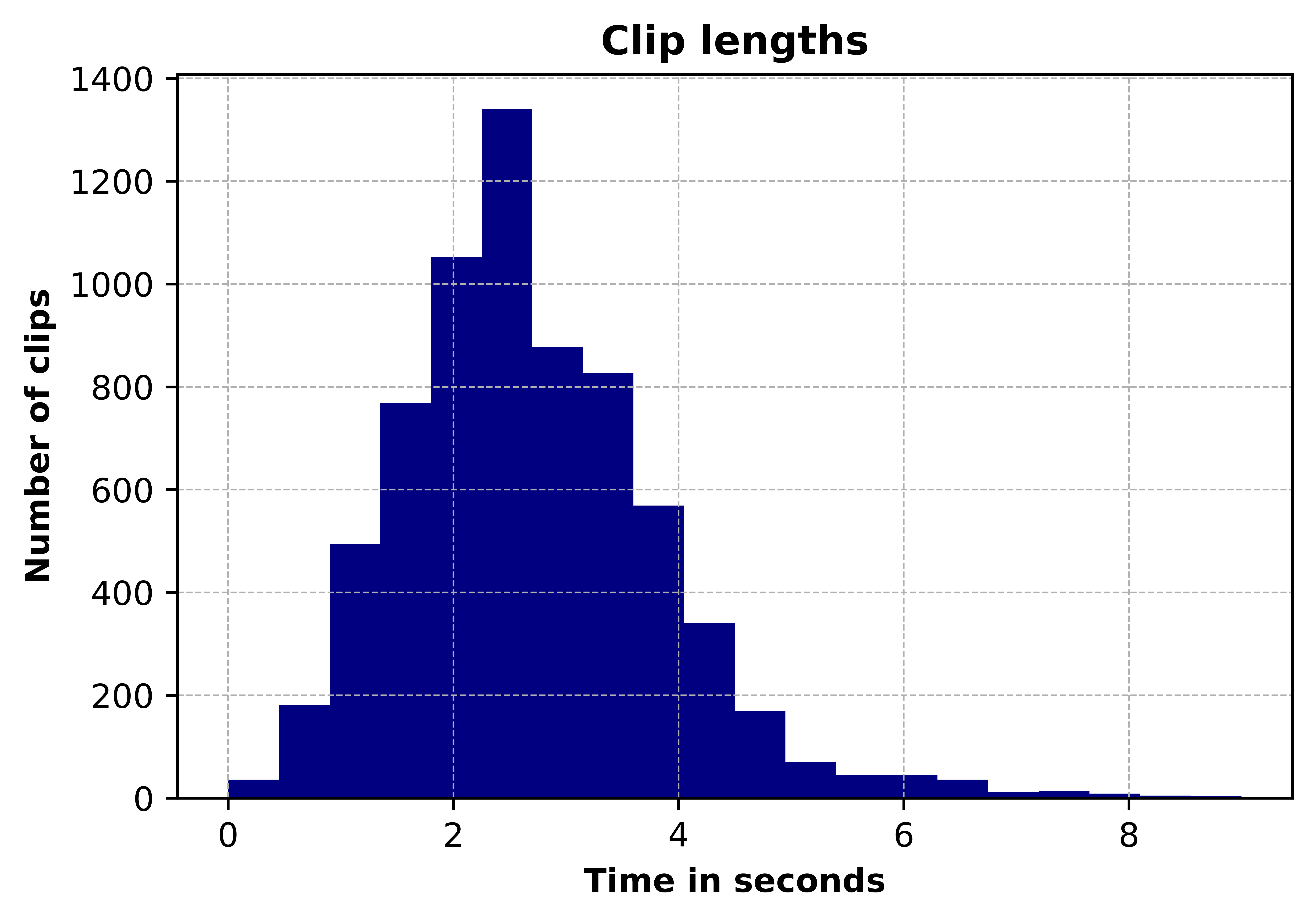
Figure 5: Distribution of clip lengths
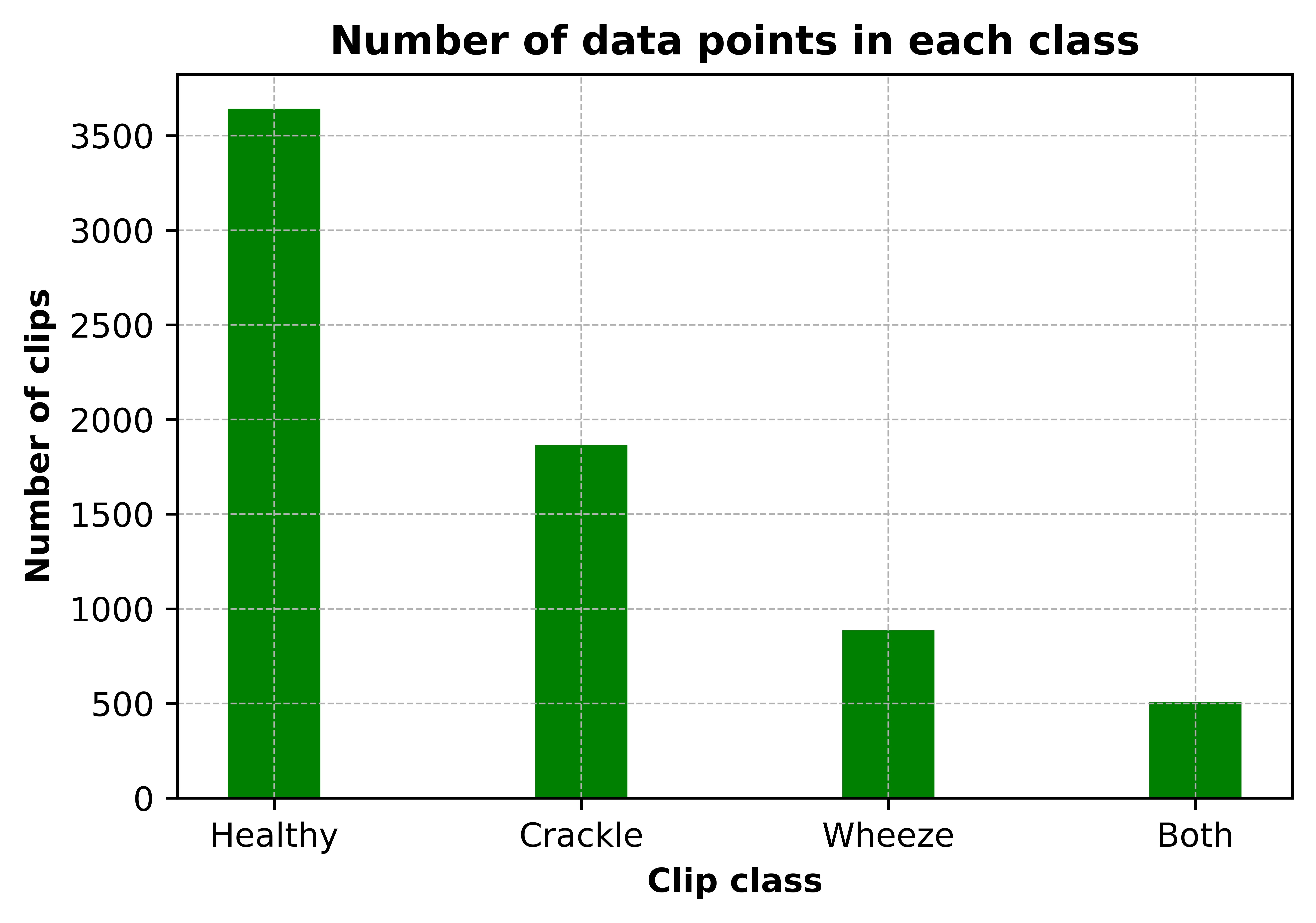
Figure 6: Class distribution of clips
Preprocessing
Preprocessing of the data starts from importing the sound files, resampling and cropping them. Since the recordings were taken by two different research teams with different recording devices, there are 3 different sampling rates (44100 Hz, 10000 Hz and 4000 Hz). All recordings were resampled to 44100 Hz and all clips are made 5 seconds long by zero padding shorter clips and cropping the longer ones. librosa library was used in this project for reading the audio data and extracting features.
Feature Extraction (MFCC)
Mel Frequency Cepstrum Coefficients were used as features of the sound clips. MFCCs are widely used in speech recognition systems. They are also being used extensively in previous work on detection of adventitious respiratory sounds as they provide a measure of short term power spectrum of time domain signals. Both the frequency and time content are important to distinguish between different adventitious sounds, since different adventitious sounds can exist in a single clip at different time periods and they differ in duration. Therefore, MFCC is helpful in capturing the change in frequency content of a signal over time. Frequencies are placed on a mel scale, which is a nonlinear scale of frequencies whose distances are percieved to be equal by the human auditory system. Output of MFCC is a 2 dimensional feature vector (time and frequency), which was then flattened into a one dimensional array before further processing. The process of calculating MFCC is given in Figure 7.
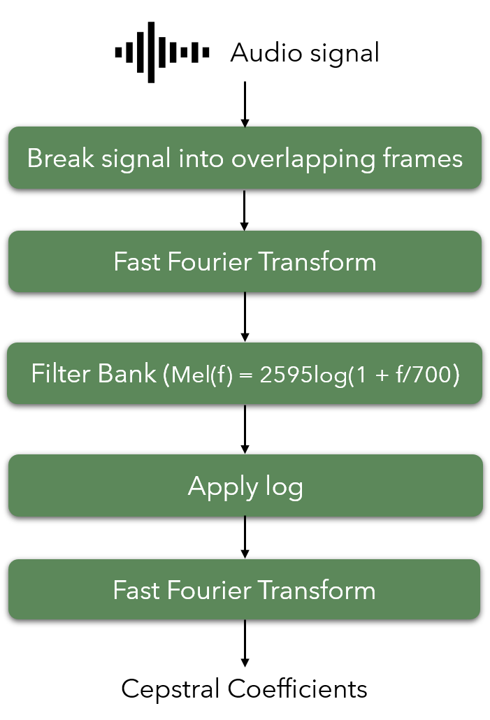
Figure 7: Flowchart of steps followed when calculating the MFCC.
A sample output of the MFCC content of clips containing different adventitious sounds is given below.
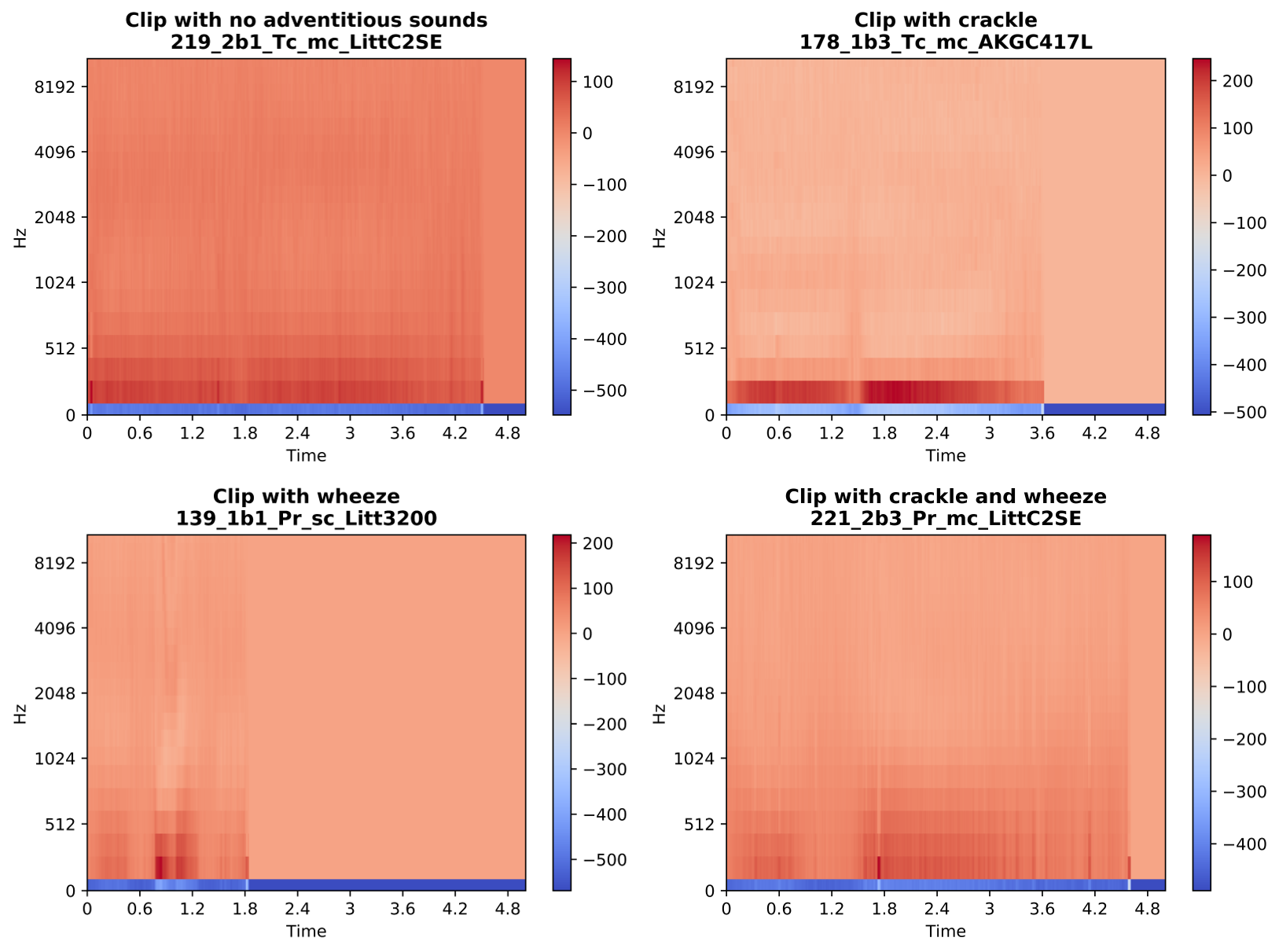
Figure 8: Sample output of MFCC of clips chosen from each class.
Dataset Partitioning
Since the dataset does not include seperate recordings for training and testing, we randomly partitioned the dataset into training (80%) and testing (20%) by maintaining the class distribution for both sets. For the first classification method (SVM), we perform a 5-fold cross validation to pick the hyperparameters, therefore, no seperate validation dataset is required. As for the second classification method (CNN), we split the training dataset so that 70% of the original dataset is used for training and 10% is used for validation. Figure 9 illustrates the class distribution for CNN system.
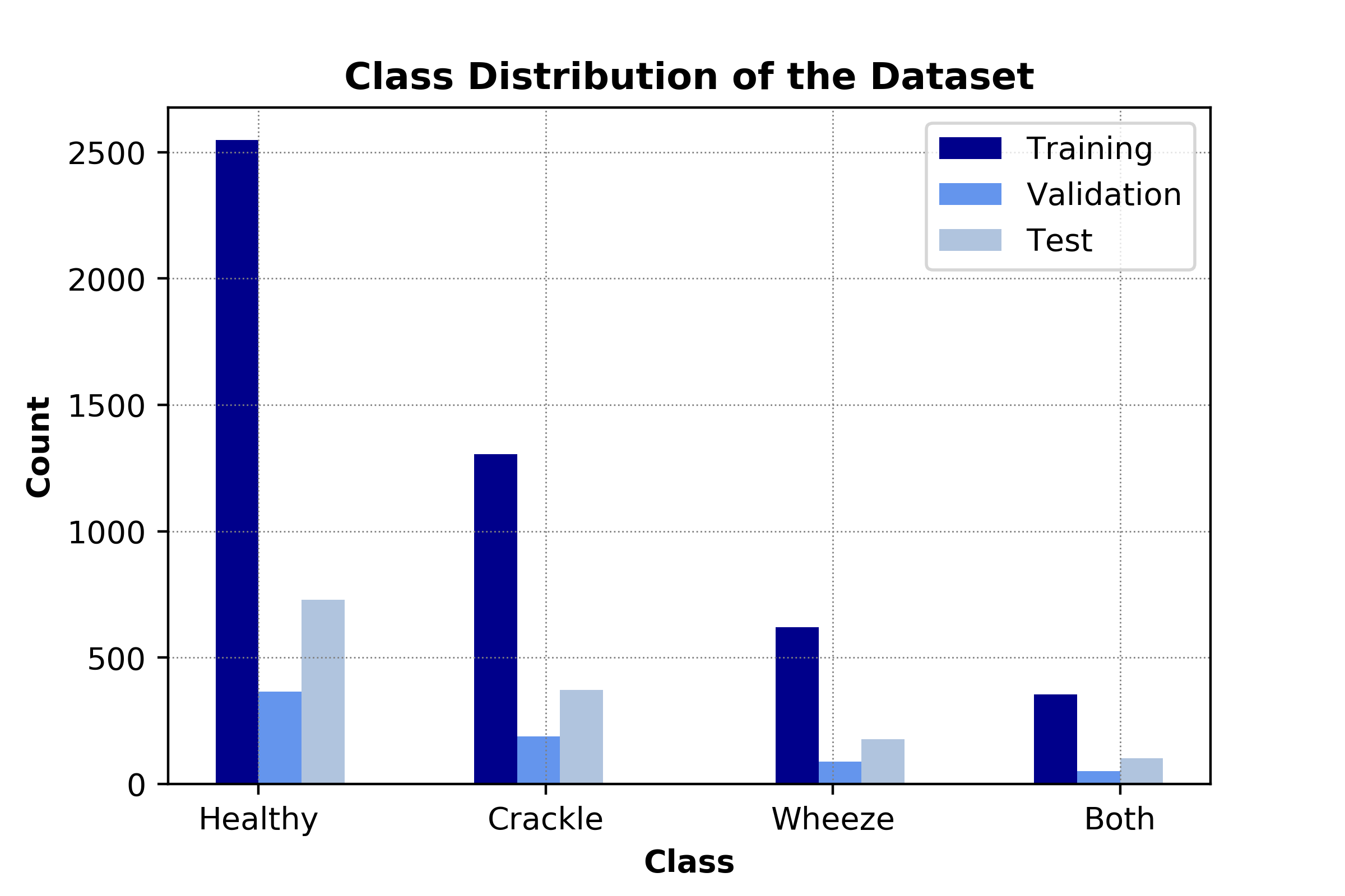
Figure 9. Distribution of the dataset to be used for CNN-based system.
Classification Methods
Principal Component Analysis (PCA) and Support Vector Machines (SVM) in Pipeline
For the first classification method of our project, we combined an unsupervised learning method, PCA, with a supervised learning method, SVM. The main reason behind including PCA before SVM was to reduce the dimensionality of the dataset and hence increase the learning rate. The details for these methods are explained next.
Principal Component Analysis (PCA) for Dimensionality Reduction
The MFCC-based features exist in a 2-dimensional space where the first and second dimensions represent the time and frequency information, respectively. Hence, the input data
where T is the number of time-windows and D is the number of frequency bins. As can be seen in the figures above, the features are sparsely distributed and most of these features show similar characteristics across different classes. This implies that the dataset contains significant amount of redundant information. In an effort to reduce the dimensionality of the dataset and hence increase the learning rate while keeping the variation within the dataset, we propose to utilize principal component analysis (PCA).
PCA is a commonly used unsupervised learning technique in machine learning that projects the dataset into a lower dimensional dataset in an optimal manner that maximizes the remained variance 31 . PCA performs a linear transformation and is therefore useful for datasets that are linearly seperable. In conventional PCA application, the input data for each sample is represented as a vector (1-dimensional). Therefore, the whole dataset can be represented as a 2-dimensional matrix that consists the stacked input vectors. Firstly, the dataset is centered to avoid a biased projection. Later, the centered data matrix is expressed in singular value decomposition form. The projection is performed by keeping the largest singular values and their corresponding eigenvectors. The number of the singular values that are utilized can be determined manually or can be chosen so that the explained variance of the original dataset achieves a certain threshold.
Our MFCC-based features lie in a 2-dimensional space. To be able to utilize the conventional PCA scheme, we flatten the features so that the features are represented as a vector. Then, we can apply the common PCA procedure. However, PCA is not agnostic to different scalings of the features. Therefore, we standardize the data so that all features are similarly scaled.
To give a perspective of the dimensions, when the maximum length of the recording are limited to 5 seconds, the resulting MFCC features have the dimension 20 x 431. Therefore, we have 8620 features in total. As explained above, the values for most of these features are the same across the different classes and redundant. In Figure 10 how the explained cumulative variance changes for increasing number of components is presented. We note that we still keep the 99% of the original variance when the dimensionality is reduced to 1916. This reduction is very significant because it becomes useful to increase the learning rate in the next step.
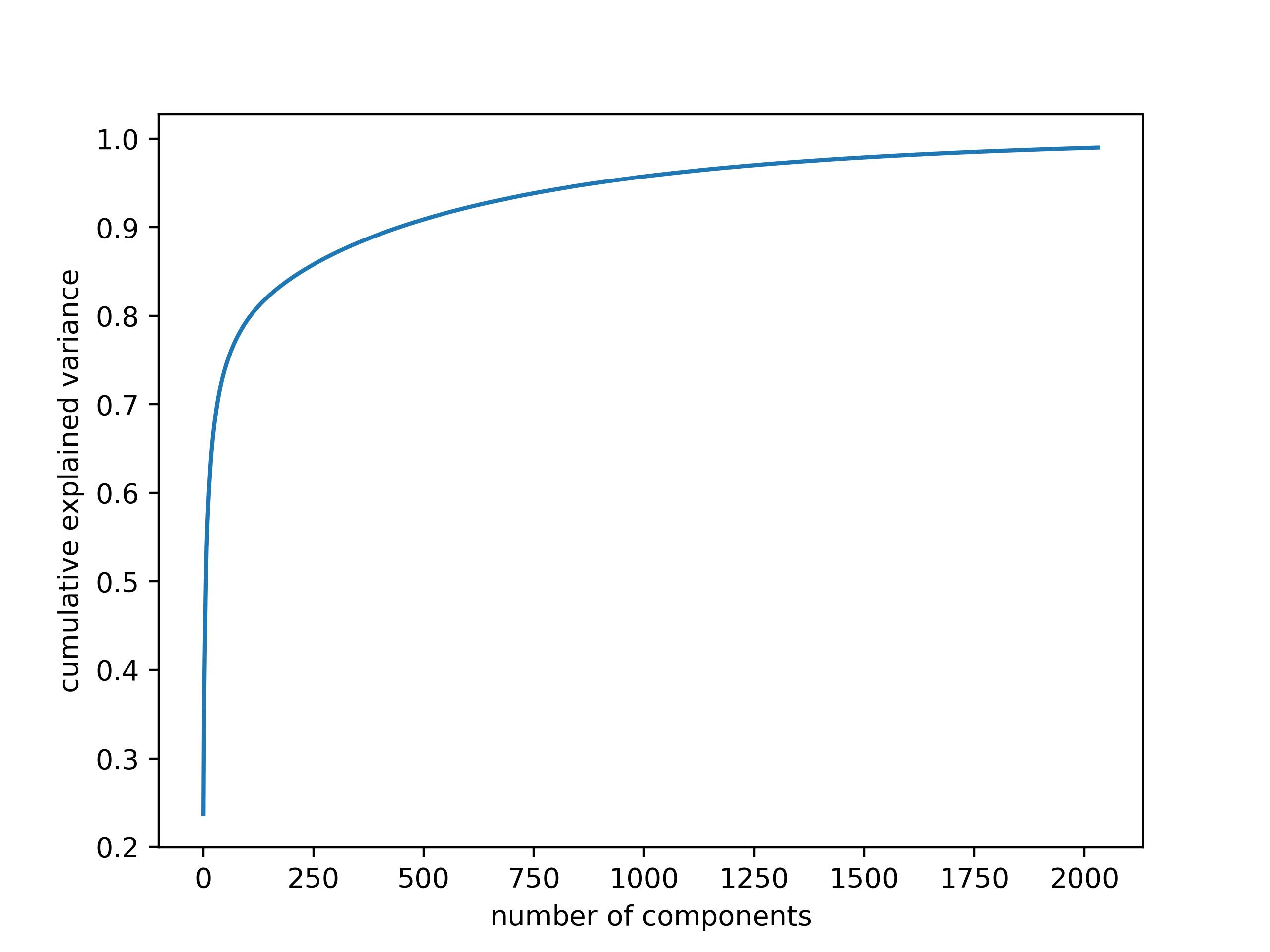
Figure 10. Explained variance for increasing number of kept principal components
Support Vector Machines (SVM)
As the first supervised classification method, we trained Support Vector Machine (SVM) for four-class classification. SVMs rely on kernel methods to adapt to patterns of data, by nonlinearly mapping the data from original space into a higher dimensional space. A key initial step in SVM is normalizing the predictor or feature space for SVM training. As discussed earlier our SVM is fed by the output of the PCA. Thus, such normalization is done as an initial step in PCA. That means the input for SVM is already normalized to standardize features. The second step is choosing kernels and regularization parameters. Although there are automated ways of doing so, we avoided such automation, to prevent any potential overfitting of the model. Since our features are nonlinearly distributed in feature space, we chose the Radial Basis Function (RBF) to enhance SVM flexibility and robustness to fit the given data distribution. Mixture of SVM and RBF requires an appropriate tuning of SVM hyperparameters.
Parameters Tuning:
The SVM parameters are determined through maximization of a margin-based criterion. This criterion is approximately optimized through two sub problems. First is related to margin maximization in the input space, and the second is related to determination of the extent of sample spread in the feature space. Thus, here our hyperparameters for SVM are: first, the soft margin parameter C in input space which is obtained by its analytical formula, second, the RBF kernel Gamma parameter in the feature space.
RBF Parameters : Gamma & C
RBF parameters are Gamma and C. Gamma reshapes a decision boundary, by trying to assemble and cluster similar data points. and C parameter is called penalty parameter which controls the penalty of misclassification.
We splitted data into training and testing partitions for cross validation with 5 folds. In setting the fitness function, we calculated the root-mean-square deviation (RMSD) of the model over the test data. RMSD quantifies the difference between model predicted values and observed value. By minimizing the RMSD value, we optimized the values of parameters Gamma and C. Discussed approaches allow us to have more robustness after cross validation, more generalization across randomly split trst samples, and less bias between prediction and actual observations. The optimized Gamma is equal to 1e-4 and C is equal to 10.
In total there were 10 candidates and 50 fits. Each fit takes about 4 minutes with total fit time about 200 minutes. The overal efficiency and accuracy result of our model is discussed in next parts.
Convolutional Neural Networks (CNN)
As the second classification approach, we propose to use a Convolutional Neural Network based system. The Convolutional Neural Network (CNN) is a neural network classification technique that is commonly used in image classification 24 28. As opposed to the traditional neural networks, where each input feature is associated with seperate parameters, in CNN, parameters are shared among the features. This allows the network for learning local features. By this means, CNN automatically learns the important features without requiring extra feature extraction. CNN-based architectures construct a deep layered structure through convolutional kernels, which are learned from the data to extract complex features. Furthermore, CNN is computationally efficient. Convolution and pooling operations allow for parameter sharing and efficient computation.
In our project, the MFCC-based features are 2-dimensional. Therefore, they can be treated as images and the assignment can be translated into an image classification task. After experimenting with commonly used CNN structures such as AlexNet 24 and VGGNet 28, we designed our own CNN-based neural network structure as shown in Figure 11.
Our network includes three convolutional layers (each followed by a max-pooling layer) and four fully connected layers as well as the output layer. The convolution operations are performed with a kernel size of 15x15 and stride of 1. The fully connected layers have 6784, 2048, 1024 and 128 neurons, respectively. The activation function for all convolutional and fully connected layers is Rectified Linear Unit (ReLU). The output layer, consisting of 4 nodes, implements a softmax activation function. The max-pooling operations are performed with a kernel of size 2x2 and stride 1.
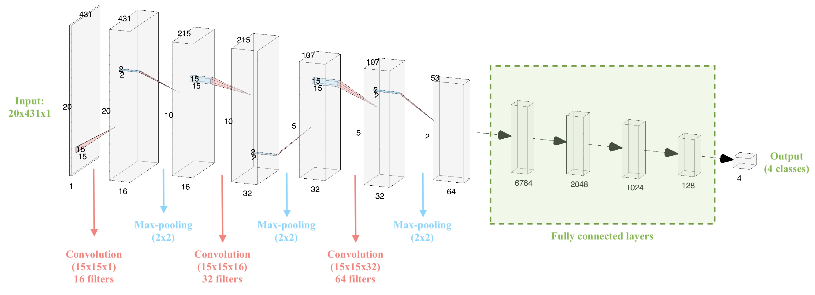
Figure 11. Architecture of the CNN-based neural network
The proposed neural network system above consists of over 16 million parameters to be trained. Considering the dataset size, this is a significantly large number of parameters. To increase the training speed, we use Adam optimizer 4. We specify our loss function as categorical cross entropy
.
where,
,
and the number of classes is C = 4. Then, we train our algorithm and evaluate it on the validation set to choose the the number of epochs.
Evaluation & Results
SVM Results
Our best SVM model achieved an accuracy of 69%. Interestingly, the recall percentages correlate well with the distribution of classes in our data. When looking at the unbalanced dataset, as less training data was available in each class, the corresponding recall values also decreased. Figure 12 is the confusion matrix with percent recall values, and Figure 13 illustrates this by normalizing the number of clips in each class and the recall of each class.
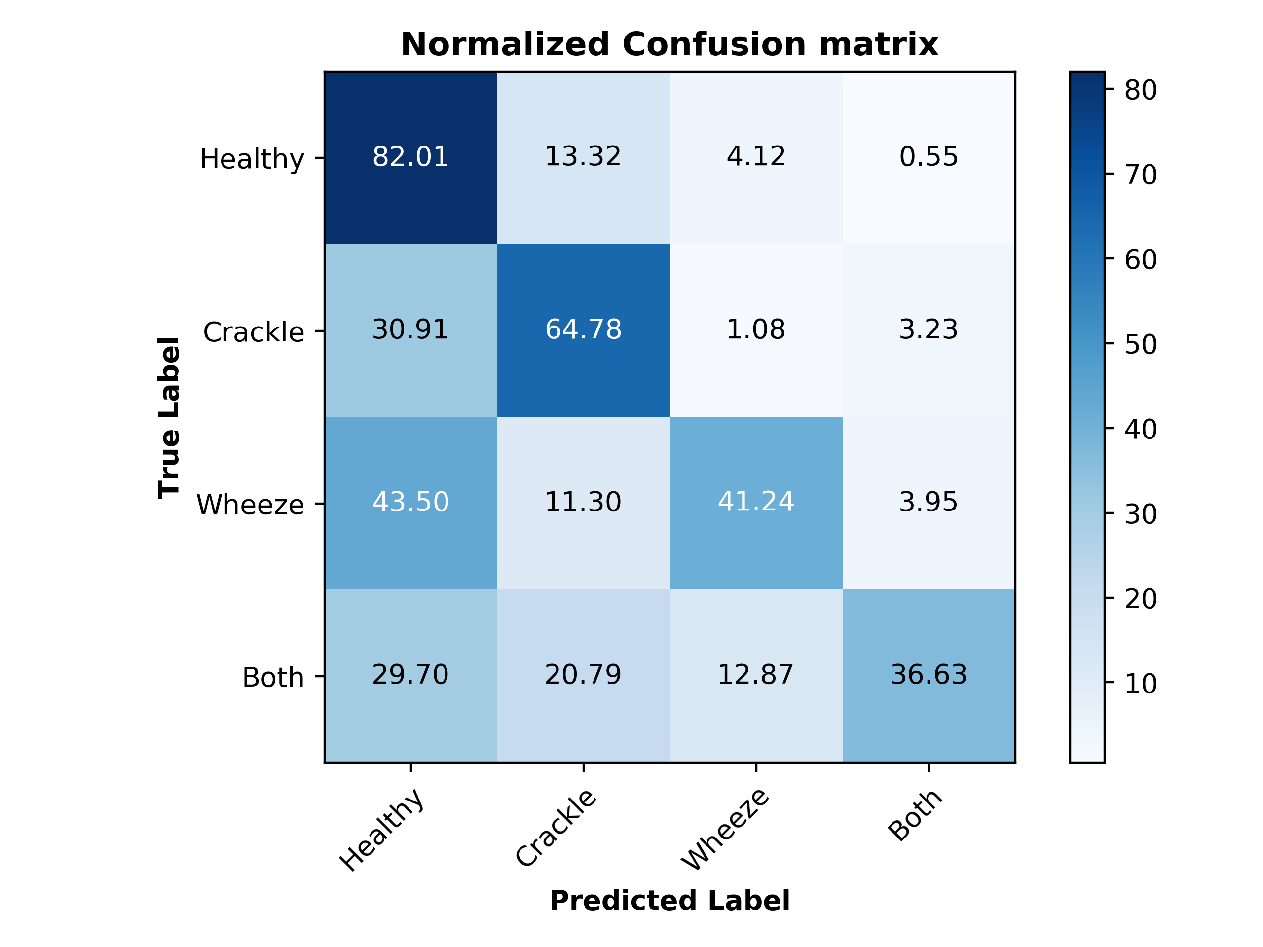
Figure 12. Normalized confusion matrix for SVM model
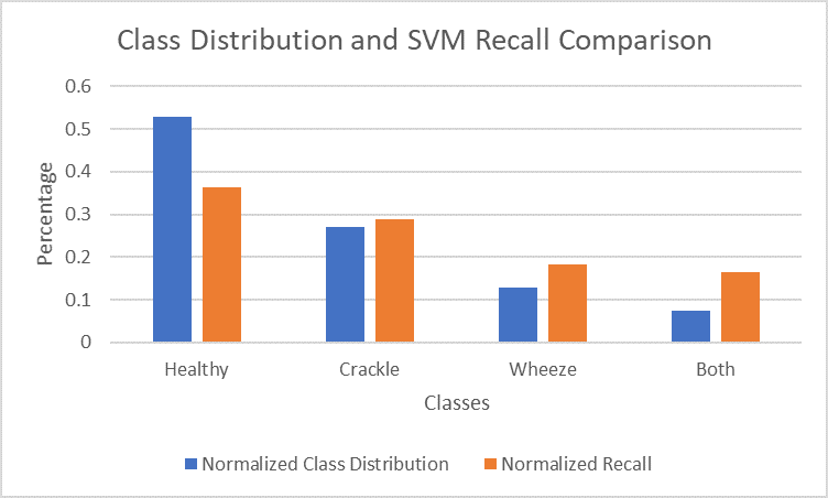
Figure 13. Comparison of normalized class distribution and normalized recall for each class in SVM model
The unbalanced data could be the reason for our relatively low accuracy of 69%. The healthy class, which had the most data available (3642 clips) achieved a recall of 82%, while the both class, with the least data available (506 clips) achieved a recall of 37%.
CNN Results
Our best CNN model achieved an accuracy of 71%. The normalized confusion matrix is shown in Figure 14.
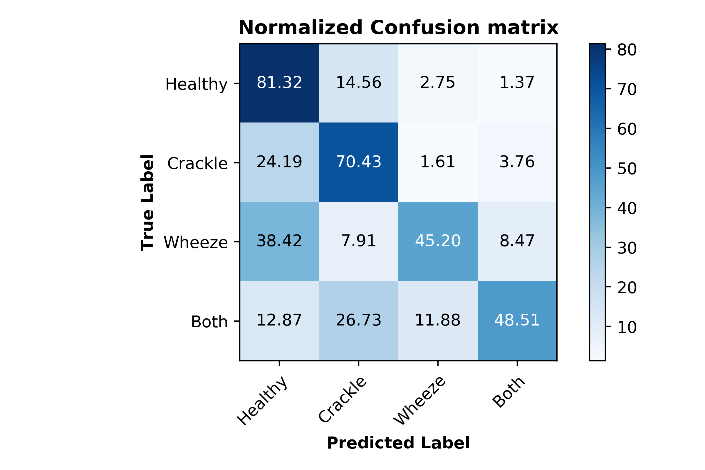
Figure 14. Normalized confusion matrix for CNN model
Like the SVM model, the recall percentages for the CNN model also correlate well with the distribution of classes in our data. The graph of the normalized class distribution and recall comparison is shown in Figure 15.
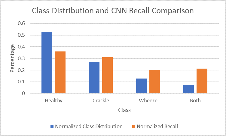
Figure 15. Comparison of normalized class distribution and normalized recall for each class in CNN model
Overfitting starts to happen at around the 20th epoch. After the 20th epoch, the testing accuracy starts to increase at a noticeably slower rate than the training accuracy. The testing loss also stops decreasing at this point, while the training loss continues to decrease. Although more training at each epoch does result in a higher validation accuracy, the accuracy gain is much less when compared to the training accuracy. A graph of the training and validation accuracy is shown in Figure 16, and a graph of the training and validation loss is shown in Figure 17.
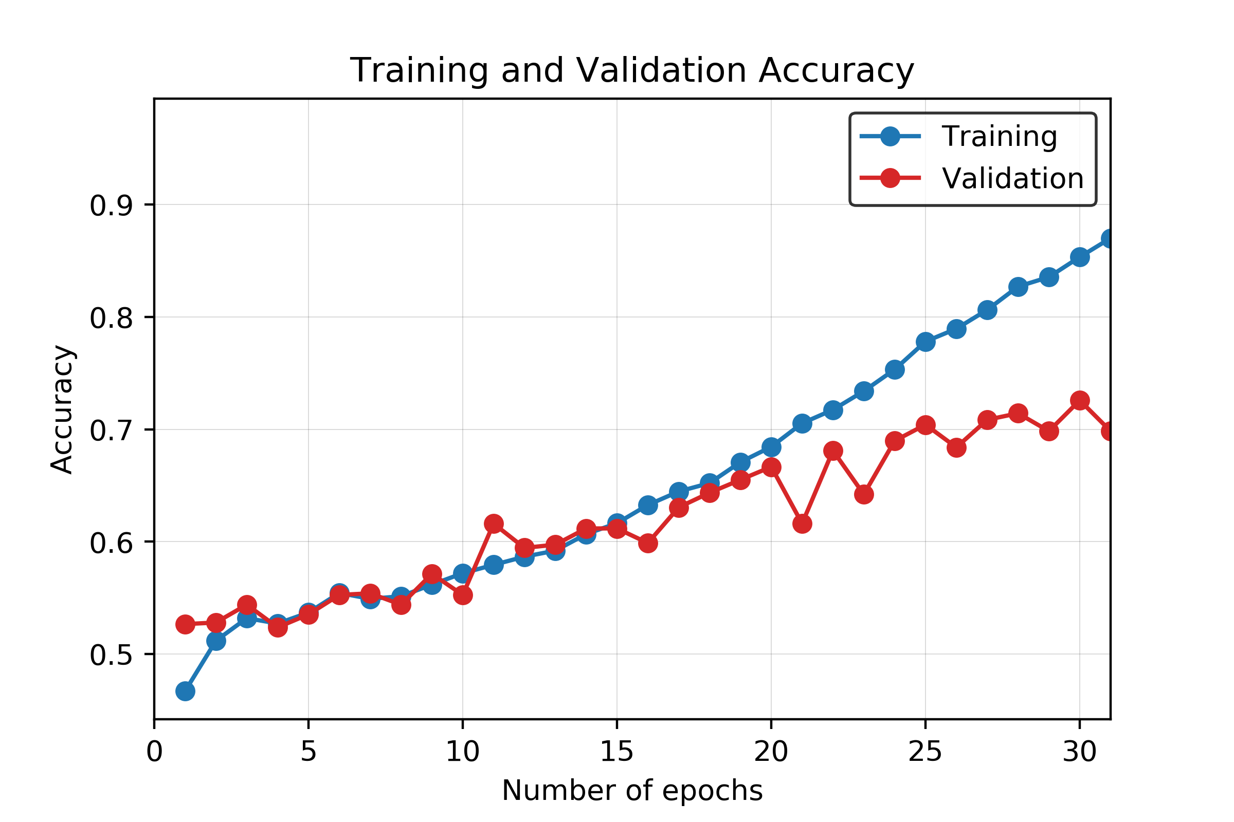
Figure 16. Training and validation accuracy for CNN model across 30 epochs
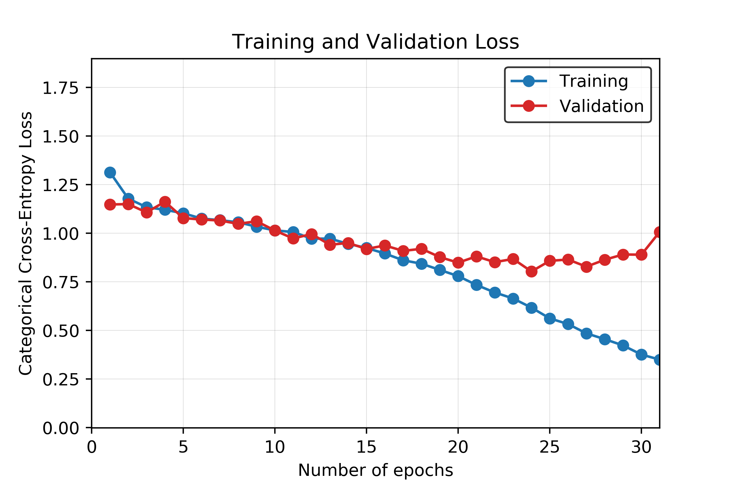
Figure 17. Training and validation loss for CNN model across 30 epochs
Dataset Evaluation and Discussion
The accuracy results of our work is significantly impacted by several factors. Those factors are 1) demographic information, 2) devices used for collecting sound data, 3)location on the body for which data is collected from and 4) unbalanced number of samples in each class as well as different time duration for each recorded sample. Since data is not categorized based on all these factors, preprocessing, feature extraction, and overall data cleaning part was very complicated. These issues have remarkably impacted the classification accuracy. We elaborate more on those factors here:
-
Demographic information includes age, sex, and body mass index (BMI). We have recordings from both genders and there are children and adults among patients. Such age, gender and BMI variations impact a lot on the time duration of each respiratory cycle.
-
The location on the body for data collection, impact the frequency profile of each sample. Our data is collected from seven different locations on the body; Trachea, Anterior left/ right, Posterior left/right, and lateral left/right. Based on our knowledge, lateral locations have lower frequency ranges compared to trachea for the same class of abnormal sounds.
-
Recording equipment is another key factor which influences the signal to noise ratio (SNR) tremendously. Our data is collected by four different equipments, while there is a huge gap among their performance. For instance, the SNR for signals collected by “3M Litmmann 3200 Electronic Stethoscope (Litt3200)” is much higher compared with the other devices.
-
The format of the data itself impacts on our final accuracy. All the clips were of different lengths, ranging from 0.2 to 16.2 seconds. The clips were also not sampled at the same sampling rate. This required us to augment the data through zero-padding, cropping, filtering, and up-sampling or down-sampling, which removed from the truth of the actual data and could cause problems in the training process.
-
Considering the number of parameters to be trained (over 16 million) in the CNN implementation, the dataset size is very small (4827 total samples) and this restricts the learning capability of the network.
To recap, it is crucial for future steps, to revise our models to account for such discussed differences. It is highly important to categorize data with more care regarding those issues, and spend more time and effort on the preprocessing phase, in the future.
The results indicate that the CNN-based classification system overperforms the SVM-based system. Considering challenges with the dataset that are presented above, in the light of other results in literature, we believe 71% accuracy is a successful result. However, there is definitely some room for improvement. Next, we present possible future directions for the project.
One possible approach is to modify the CNN structure. We tried different kernel sizes (3x3, 5x5, and 11x11), but the accuracy results turned out to be comparable. Therefore, we reported the results for only the best performing kernel size (15x15). Furthermore, since the dataset is limiting the learning capability of the CNN, a transfer learning approach might be implemented, and the classification segments of the new network can be customized for this specific application.
In addition to the 2-dimensional CNN, we tried to use 1 dimensional CNN. For that, we used two different input types: 1) Flattened MFCC coefficients of size 8620x1, 2) Features obtained after applying PCA (1916x1). Training the former network took significantly long amount of time (300 s/epoch) since it required training 71 million parameters. The highest accuracy achieved with such a structure was 63%. On the other hand, training the second network took considerably less time (70 s/epoch) at the expense of significantly lower accuracy (54%). These results indicate that 2-dimensional CNN structure outperforms 1 dimensional CNN structures for this dataset.
Possible considerations to increase the performance of the system are listed as follows:
- Using a larger dataset that has a balanced class distribution,
- Utilizing other feature extraction methods such as short-time Fourier transform (STFT),
- Applying advanced signal processing techniques to extract more informative and distinctive features from the recordings,
- Incorporating a Recurrent Neural Network (RNN)-based structure to address the temporal dynamic behavior.
Conclusion
Respiratory sounds are shown to be key factors in diagnosing pulmonary diseases. Automating the process of detection and classification of the respiratory sounds promises great advantages in early diagnosis and treatment of such diseases. In this project, we studied respiratory sound classification based on the presence of adventitious sounds such as wheeze and crackle. To do so, we utilized the Respiratory Sound Database 24 that includes recordings from patients that are labeled by medical doctors. Considering different frequency spectrum characteristics of these adventitious sounds, we extracted features from the recordings by using MFCC. For classifying the samples, we implemented two different approaches. First approach consists of flattening the MFCC coefficients, applying PCA to reduce the dimensionality and finally applying SVM. Second approach utilizes a CNN-based neural network structure by treating the problem as an image classification task. We obtained 69% and 71% accuracies with the first and second approaches, respectively. Considering the challenges that the dataset has, we believe these results are relatively successful. In the discussion part, we proposed future directions that can possible increase the accuracy.
References
[1] Bhateja, Vikrant, Ahmad Taquee, and Dilip Kumar Sharma. 2019. “Pre-Processing and Classification of Cough Sounds in Noisy Environment Using SVM.” 2019 4th International Conference on Information Systems and Computer Networks (ISCON). https://doi.org/10.1109/iscon47742.2019.9036277.
[2] Chambres, Gaetan, Pierre Hanna, and Myriam Desainte-Catherine. 2018. “Automatic Detection of Patient with Respiratory Diseases Using Lung Sound Analysis.” 2018 International Conference on Content-Based Multimedia Indexing (CBMI). https://doi.org/10.1109/cbmi.2018.8516489.
[3] Chen, Hai, Xiaochen Yuan, Zhiyuan Pei, Mianjie Li, and Jianqing Li. 2019. “Triple-Classification of Respiratory Sounds Using Optimized S-Transform and Deep Residual Networks.” IEEE Access. https://doi.org/10.1109/access.2019.2903859.
[4] Chowdhury, S. K., and A. K. Majumder. 1982. “Frequency Analysis of Adventitious Lung Sounds.” Journal of Biomedical Engineering. https://doi.org/10.1016/0141-5425(82)90048-6.
[5] Cinkooglu, Akin, Department of Radiology, Ege University School of Medicine, Izmir, Turkey, Selen Bayraktaroglu, Recep Savas, et al. 2020. “Lung Changes on Chest CT During 2019
[6] Novel Coronavirus (COVID-19) Pneumonia.” European Journal of Breast Health. https://doi.org/10.5152/ejbh.2020.010420.
[7] Cugell, David, Noam Gavriely, and Dan Zellner. 2012. “Lung Sounds and the Stethoscope — a Lung Sounds Primer.” MedEdPORTAL. https://doi.org/10.15766/mep_2374-8265.9066.
[8] Devangan, Hupendra, Nitin Jain, and Chouksey Engineering College Bilaspur India. 2015. “A Review on Classification of Adventitious Lung Sounds.” International Journal of Engineering Research and. https://doi.org/10.17577/ijertv4is051274.
[9] García-Ordás, María Teresa, José Alberto Benítez-Andrades, Isaías García-Rodríguez, Carmen Benavides, and Héctor Alaiz-Moretón. 2020. “Detecting Respiratory Pathologies Using Convolutional Neural Networks and Variational Autoencoders for Unbalancing Data.” Sensors 20 (4). https://doi.org/10.3390/s20041214.
[10] İçer, Semra, and Şerife Gengeç. 2014. “Classification and Analysis of Non-Stationary Characteristics of Crackle and Rhonchus Lung Adventitious Sounds.” Digital Signal Processing. https://doi.org/10.1016/j.dsp.2014.02.001.
[11] Kingma, Diederik P., and Jimmy Ba. “Adam: A method for stochastic optimization.” arXiv preprint arXiv:1412.6980 (2014).
[12] Lehrer, Steven. 2018. Understanding Lung Sounds: Third Edition. Steven Lehrer.
[13] Liu, Renyu, Shengsheng Cai, Kexin Zhang, and Nan Hu. 2019. “Detection of Adventitious Respiratory Sounds Based on Convolutional Neural Network.” 2019 International Conference on Intelligent Informatics and Biomedical Sciences (ICIIBMS). https://doi.org/10.1109/iciibms46890.2019.8991459.
[14] Makic, Mary Beth Flynn. 2020. “Prone Position of Patients with COVID-19 and Acute Respiratory Distress Syndrome.” Journal of PeriAnesthesia Nursing. https://doi.org/10.1016/j.jopan.2020.05.008.
[15] Marini, John J., and Luciano Gattinoni. 2020. “Management of COVID-19 Respiratory Distress.” JAMA. https://doi.org/10.1001/jama.2020.6825.
[16] Marques, Alda, and Ana Oliveira. 2018. “Normal Versus Adventitious Respiratory Sounds.” Breath Sounds. https://doi.org/10.1007/978-3-319-71824-8_10.
[17] Nakamura, Naoki, Masaru Yamashita, and Shoichi Matsunaga. 2016. “Detection of Patients Considering Observation Frequency of Continuous and Discontinuous Adventitious Sounds in Lung Sounds.” 2016 38th Annual International Conference of the IEEE Engineering in Medicine and Biology Society (EMBC). https://doi.org/10.1109/embc.2016.7591472.
[18] Ntalampiras, Stavros, and Ilyas Potamitis. 2019. “Classification of Sounds Indicative of Respiratory Diseases.” Engineering Applications of Neural Networks. https://doi.org/10.1007/978-3-030-20257-6_8.
[19] Okubo, Takanori, Masaru Yamashita, Katsuya Yamauchi, and Shoichi Matsunaga. 2013. “Modeling Occurrence Tendency of Adventitious Sounds and Noises for Detection of Abnormal Lung Sounds.” https://doi.org/10.1121/1.4800330.
[20] Pan, Feng, Tianhe Ye, Peng Sun, Shan Gui, Bo Liang, Lingli Li, Dandan Zheng, et al. 2020. “Time Course of Lung Changes at Chest CT during Recovery from Coronavirus Disease 2019 (COVID-19).” Radiology 295 (3): 715–21.
[21] Perna, Diego. 2018. “Convolutional Neural Networks Learning from Respiratory Data.” 2018 IEEE International Conference on Bioinformatics and Biomedicine (BIBM). https://doi.org/10.1109/bibm.2018.8621273.
[22] Ploysongsang, Yongyudh, Vijay K. Iyer, and Panapakkam A. Ramamoorthy. 1991. “Reproducibility of the Vesicular Breath Sounds in Normal Subjects.” Respiration. https://doi.org/10.1159/000195918.
[23] Pramono, Renard Xaviero Adhi, Stuart Bowyer, and Esther Rodriguez-Villegas. 2017. “Automatic Adventitious Respiratory Sound Analysis: A Systematic Review.” PloS One 12 (5): e0177926.
[24] Krizhevsky, Alex, Ilya Sutskever, and Geoffrey E. Hinton. “Imagenet classification with deep convolutional neural networks.” Advances in neural information processing systems. 2012.
[25] Rocha, B. M., D. Filos, L. Mendes, I. Vogiatzis, E. Perantoni, E. Kaimakamis, P. Natsiavas, et al. 2018. “Α Respiratory Sound Database for the Development of Automated Classification.” Precision Medicine Powered by pHealth and Connected Health. https://doi.org/10.1007/978-981-10-7419-6_6.
[26] Saraiva, A., D. Santos, A. Francisco, Jose Sousa, N. Ferreira, Salviano Soares, and Antonio Valente. 2020. “Classification of Respiratory Sounds with Convolutional Neural Network.” Proceedings of the 13th International Joint Conference on Biomedical Engineering Systems and Technologies. https://doi.org/10.5220/0008965101380144.
[27] Sawant, R. K., and A. A. Ghatol. 2015. “Classification of Respiratory Diseases Using Respiratory Sound Analysis.” International Journal of Signal Processing Systems. https://doi.org/10.12720/ijsps.4.1.62-66. Scott, Gregory, Edward J. Presswood, Boikanyo Makubate, and Frank Cross. 2013. “Lung Sounds: How Doctors Draw Crackles and Wheeze.” Postgraduate Medical Journal. https://doi.org/10.1136/postgradmedj-2012-131410.
[28] Simonyan, Karen, and Andrew Zisserman. “Very deep convolutional networks for large-scale image recognition.” arXiv preprint arXiv:1409.1556 (2014).
[29] Spieth, P. M., and H. Zhang. 2011. “Analyzing Lung Crackle Sounds: Stethoscopes and beyond.” Intensive Care Medicine. https://doi.org/10.1007/s00134-011-2292-3.
[30] Vrbancic, Grega, Iztok Jr Fister, and Vili Podgorelec. 2019. “Automatic Detection of Heartbeats in Heart Sound Signals Using Deep Convolutional Neural Networks.” Elektronika Ir Elektrotechnika. https://doi.org/10.5755/j01.eie.25.3.23680.
[31] Wold, Svante, Kim Esbensen, and Paul Geladi. “Principal component analysis.” Chemometrics and intelligent laboratory systems 2.1-3 (1987): 37-52.
[32] Xu, Zhe, Lei Shi, Yijin Wang, Jiyuan Zhang, Lei Huang, Chao Zhang, Shuhong Liu, et al. 2020. “Pathological Findings of COVID-19 Associated with Acute Respiratory Distress Syndrome.” The Lancet. Respiratory Medicine 8 (4): 420–22.